
Coldbridge
Psi-Value Calculator
A two-dimensional steady-state thermal bridging solver to ISO 10211. Draw the detail, set the boundary conditions, and get a linear transmittance you can document — ahead of the NECB Tier 2 deadline in April 2027.
Designed by a practising P.Eng for energy advisors, energy engineers and building consultants.
Thermal bridging without the overhead
Psi-value calculations sit on the critical path for NECB Tier 2 compliance, and the established tools were built for a different era of practice. This one runs in a browser, opens instantly, and is built around how the calculation is actually used in a working day.
Draw the section with rectangles or polygons, or trace over a scanned drawing by calibrating one known length. Assign materials from the library, mark the internal and external boundary conditions, and unmarked surfaces are treated as adiabatic cut-off planes. Enter flanking element U-values and lengths, and the solver returns Ψ = L2D − ΣU·L.
Since NECB 2017, Article 3.1.1.7 has required the overall thermal transmittance of envelope assemblies to account for thermal bridging, including major junctions such as slab edges, balconies and parapets. Coldbridge produces the Ψ-values that calculation needs.
Not engineering advice. The calculator is a tool. You remain the responsible professional and must independently verify all results before relying on them in a submission or a design decision.
$30 CAD / month
Billed monthly. Cancel any time.
or $290 a year — the equivalent of $24.17 a month, with just over two months free.
Unlimited calculations
Run as many details as your projects need.
Documented output
Formatted reports recording inputs, method and result.
Saved projects
Your work is kept against your account across devices.
Try it free for 30 days
Tell us a bit about your work and we’ll email you a trial code within one business day. If you have a detail on the go, mention it and we’ll walk through it with you.
Checked against the standard’s own test cases
ISO 10211:2017 Annex C sets out reference cases with published answers, so any solver claiming conformity can be measured rather than trusted. Both two-dimensional cases are built into the software under the Verify menu. You can run them yourself.
| Reference case | Result | Permitted |
|---|---|---|
| Case 1 — 28 reference temperatures | Max deviation 0.005 °C | ±0.1 °C |
| Case 2 — heat flow rate | 9.49 W/m against 9.5 W/m | ±0.1 W/m |
| Case 2 — 9 surface temperatures | Max deviation 0.039 °C | ±0.1 °C |
| One-dimensional wall — Ψ must be zero | Matches the analytical U-value | exact |
Case 2, point by point (°C):
| Point | A | B | C | D | E | F | G | H | I |
|---|---|---|---|---|---|---|---|---|---|
| Annex C | 7.1 | 0.8 | 7.9 | 6.3 | 0.8 | 16.4 | 16.3 | 16.8 | 18.3 |
| Coldbridge | 7.06 | 0.76 | 7.89 | 6.27 | 0.83 | 16.41 | 16.33 | 16.77 | 18.33 |
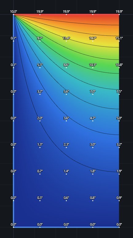
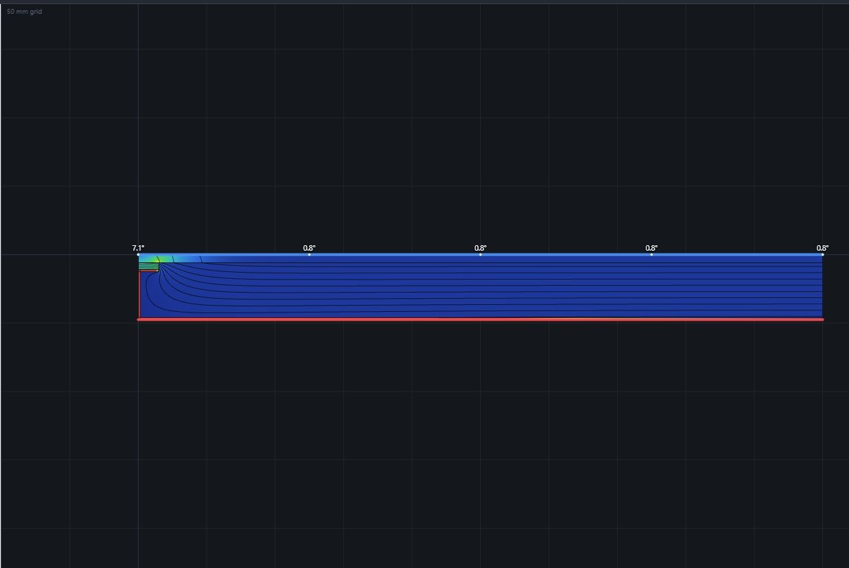
Solver
Finite-volume discretisation on a uniform Cartesian grid, solved with a preconditioned conjugate gradient method.
Mesh used
Case 1 at 2.5 mm cells (80,000 unknowns), case 2 at 0.5 mm to resolve the aluminium sheet (95,000 unknowns).
Energy balance
Heat-flow balance error of 4.7×10⁻⁷ % on case 1 and 9.9×10⁻⁹ % on case 2, well inside the 1 % the standard allows.
A mesh refinement check is built in: halve the cell size and compare, as ISO 10211 §5.3 requires for demonstrating an adequately fine grid.
Intermediate floor at an insulated cavity wall
A reinforced concrete floor slab bearing on the inner leaf of a cavity wall, with the cavity insulation running unbroken past the slab. The question is how much the floor costs you in extra heat loss, and whether the inside face stays warm enough to avoid condensation.
Model
| Layer | λ W/(m·K) |
|---|---|
| Brick, outer leaf | 0.77 |
| Mineral wool, full-fill cavity | 0.038 |
| Aircrete block, inner leaf | 0.16 |
| Gypsum plaster | 0.57 |
| Floor slab, dense reinforced concrete | 2.3 |
| Cement screed | 1.15 |
Boundary conditions 20 °C internal and 0 °C external, with Rsi = 0.13 and Rse = 0.04 m²K/W. One flanking element, the external wall at U = 0.28 W/m²K over the 2.4 m modelled height, giving ΣU·l = 0.6720 W/(m·K).
Solved on an automatic mesh of 606 × 960 cells at 2.5 mm, 171,840 unknowns, converging in 1,471 iterations to a residual of 1×10⁻⁹ with a heat-flow balance error of 4.5×10⁻⁸ %.
Ψ and fRsi are both independent of the boundary temperatures chosen, so these figures carry to any design condition. The absolute surface temperature does not.
0.015 W/(m·K)
Linear thermal transmittance Ψ
| L2D thermal coupling | 0.6869 |
| Σ U·l | 0.6720 |
| Heat flow Q | 13.74 W/m |
| fRsi at Rsi 0.25 | 0.932 |
Download the sample report (PDF)
What is in the tool
Geometry
Rectangle and polygon drawing on a snapping grid, with pan, probe and fit. Load a photo or PDF export as a reference image, calibrate one known length, and trace the section over it.
Materials
A conductivity library covering masonry, concrete and common assembly materials, with custom and composite materials, plus import and export so a library moves between machines.
Boundary conditions
Internal and external surface lines with configurable Rsi and Rse. Unmarked surfaces default to adiabatic, matching the ISO 10211 cut-off plane convention.
Solver and mesh
Finite-volume solution on an automatic or manually set cell size, so you can trade resolution against solve time on a complex detail.
Results
Temperature field with isotherms, and fRsi evaluated at Rsi = 0.25 for condensation risk assessment alongside the psi-value.
Flanking elements
Enter U-values and lengths per element, with ISO 13370 handling for ground-coupled details. Lengths follow whichever dimension system your U-value areas use.
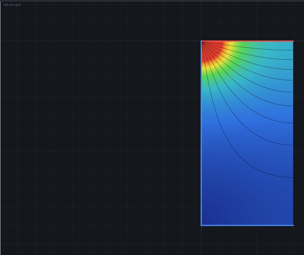

Either field can be displayed for any model, with isotherms and a readable temperature grid at a spacing you set.
Common questions
Where is my project data stored?
The solver runs in your browser. Saved projects and any custom materials you add to your library are stored in our database with our web host, Hostinger, on servers in the United States (Massachusetts), with backups in Boston. Payments are handled by Stripe and PayPal; we never see your card number. See the privacy policy for details.
What does the report contain?
Inputs, materials and conductivities, boundary conditions, mesh, energy balance and the result, as a printable report you can save as a PDF from your browser’s print dialog. Download the sample report to see one.
Which browsers does it run in?
Current Chrome, Edge, Firefox and Safari on a desktop or laptop. Tablets and phones are not supported yet.
Can my firm buy several seats?
Each subscription covers one user. For several people, each takes their own subscription. Sharing one login is not permitted.
How do I cancel?
From your Account page. Access continues to the end of the period you paid for. Any charge can be refunded within 3 days under the refund policy.
What happens to my saved projects if I cancel?
They stay on your account; cancelling ends access, not your data. Subscribe again and they’re all there. You can also use Save to download any project as a file at any time, and Export library to keep your custom materials. To have everything deleted, email us.
Is it ISO 10211 compliant?
It is validated against the ISO 10211:2017 Annex C two-dimensional reference cases, and you can run them yourself under Verify. The results table above shows every deviation.
Questions before you subscribe?
Get in touch and we will walk you through what the calculator does and whether it fits your workflow.